A camera does something deceptively simple: it turns light into numbers. The scene in front of it — a street, a face, a handwritten digit — arrives in memory as a grid of pixel values, and nothing about that grid knows it contains a street or a face. Computer vision is the discipline of turning those numbers back into meaning. Everything downstream — self-driving perception, medical imaging, the autofocus on your phone — is some version of that one translation.
An image is a grid of numbers
Start with the substrate. A grayscale image is a two-dimensional array: each cell holds one number, the brightness at that point, usually from 0 (black) to 255 (white). A colour image is three of those arrays stacked — one each for red, green, and blue — so a modest 1000×1000 photo is three million numbers. That is the entire raw input. There is no "edge," no "cat," no "road sign" written anywhere in it; those are patterns we read out of the arrangement of values.
The core reframing
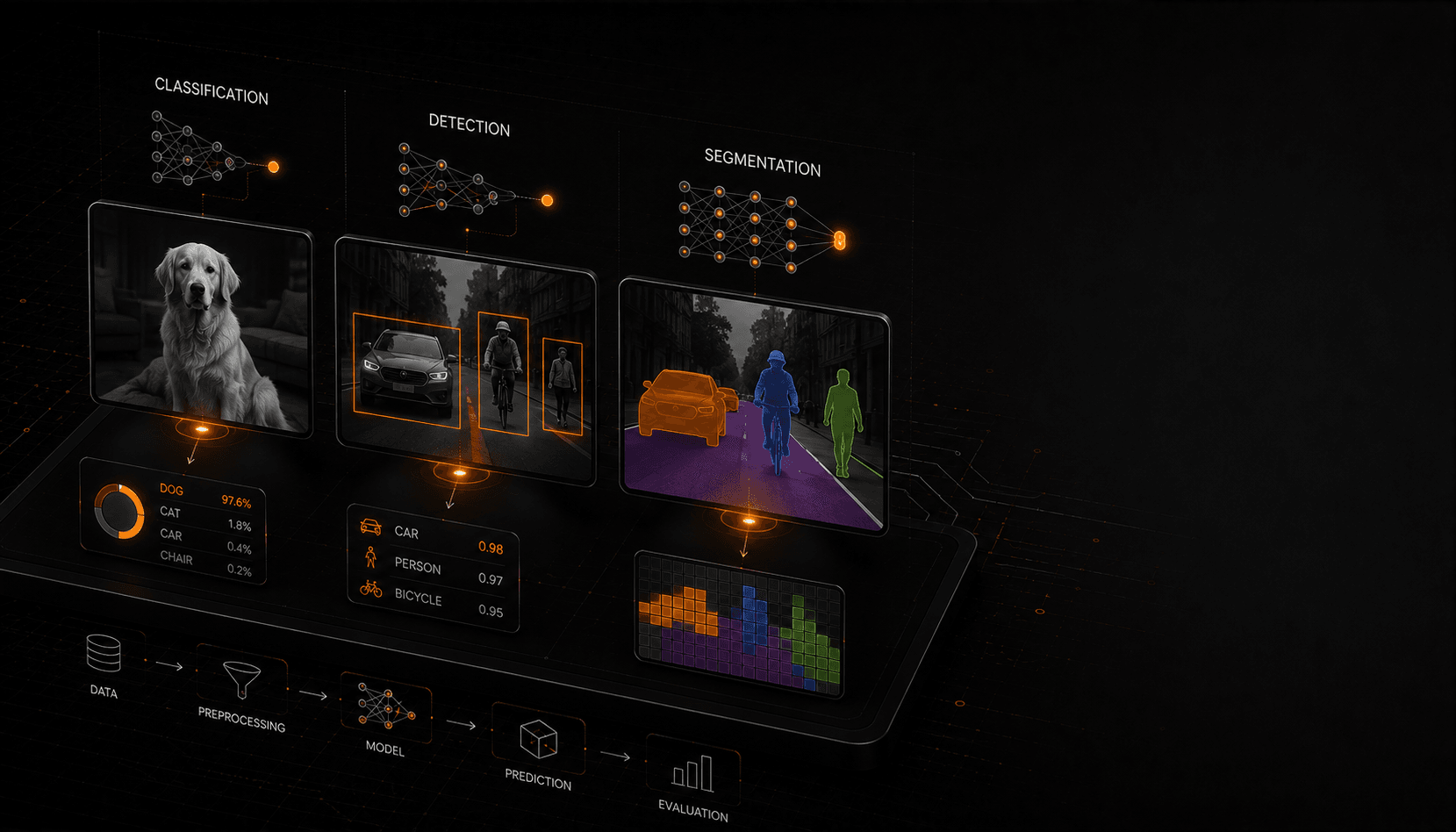
Every computer-vision task is a function that maps a large, low-level array of pixels to a small, high-level piece of structure. Classification maps it to one label. Detection maps it to a set of boxes. Segmentation maps it to a per-pixel labelling. The art is in the middle.
That reframing is worth holding onto, because it explains why raw pixels are a terrible thing to compare directly. Two photos of the same cat — one a few pixels shifted, or a shade brighter — differ in almost every single value, even though they mean the same thing. So the first job of any vision system is to convert fragile pixel values into more stable features.
Convolution: the one operation to understand
The workhorse that does that conversion is convolution. The idea is small enough to hold in your head: take a tiny grid of weights called a kernel (say 3×3), slide it across every position in the image, and at each spot multiply the kernel against the pixels underneath it and sum the result. That single number becomes one pixel of a new image — a feature map that highlights wherever the kernel's pattern appears.
Different kernels detect different things. A kernel with a strong negative-to-positive gradient across it lights up on vertical edges; rotate it and it finds horizontal ones; other kernels blur, sharpen, or pick out texture.
import numpy as np

# A 3x3 Sobel kernel: responds strongly to vertical intensity edges.
sobel_x = np.array([[-1, 0, 1],
                    [-2, 0, 2],
                    [-1, 0, 1]])

def apply_kernel(patch, kernel):
    # Multiply the kernel elementwise over one image patch, then sum.
    return float((patch * kernel).sum())

# Slide `sobel_x` over every 3x3 neighbourhood of an image and you get an
# "edge map": bright where brightness changes fast, dark where it is flat.
# Stack many such maps and you have described the image by its structure,
# not its raw pixels.
Convolution has two properties that make it the right tool. It is local — each output depends only on a small neighbourhood, matching how visual structure actually works — and it is translation-equivariant: the same edge detector fires whether the edge is in the top-left or the bottom-right. That is exactly the invariance raw pixel comparison lacked.
The shift that changed everything: learned filters
For decades, engineers designed those kernels by hand — Sobel for edges, Gaussians for blur, hand-tuned banks of filters feeding a separate classifier. It worked, but every new problem meant a new round of manual feature engineering.
The modern era began when people stopped hand-designing filters and let the network learn them. A convolutional neural network stacks many convolution layers; the kernel weights are not chosen by a person but discovered by training against labelled examples. Early layers converge on edge and colour detectors; middle layers combine those into textures and motifs; late layers respond to whole objects. The same machinery that once took a research team to design now falls out of gradient descent.
The turning point is usually dated to the 2012 ImageNet competition, where a deep convolutional network cut the image-classification error rate dramatically past every hand-engineered approach — and the field reorganised around learned features almost overnight. The lesson generalised: given enough labelled data and compute, learned representations beat hand-crafted ones. Nearly every vision system built since rests on that result.
The three things vision systems do
Once you can extract good features, the "task head" on top decides what kind of answer you get. It is worth knowing the taxonomy, because picking the wrong one is a common early mistake:
| Task | Question it answers | Output |
|---|---|---|
| Classification | What is in this image? | One label (+ confidence) |
| Detection | What is here, and where? | Boxes with labels |
| Segmentation | Which pixels belong to what? | A per-pixel mask |
These are increasingly precise — and increasingly expensive to label and train. I dig into how each one works, and the model families behind them, in a companion piece on classification, detection, and segmentation. For now the point is that "computer vision" is not one problem; it is a ladder of them, and you climb only as high as your problem actually needs.
Where vision quietly breaks
The failure modes are as important as the capabilities, because a vision model fails confidently — it returns a crisp answer even when it is wrong.
Pros
- Superhuman on narrow, well-represented tasks (reading digits, sorting defects, matching faces in good light).
- Learned features transfer: a network trained on millions of images is a strong starting point for a new task with far less data.
- Runs in real time on modest hardware once trained, including increasingly on-device.
Cons
- Distribution shift: performance falls off a cliff on lighting, angles, or object types unlike the training set.
- Data hunger: strong models need large, well-labelled datasets, and labels for detection and segmentation are costly.
- Adversarial and edge inputs: small, deliberate perturbations — or just weird real-world scenes — can flip a prediction with high confidence.
The distribution is the product
Most vision projects live or die on data, not architecture. A model trained on daytime, front-facing, well-lit images will look excellent in the demo and fail on the night shot, the odd angle, the occluded object. Before tuning the network, ask what your real inputs look like — and make sure the training set looks like them.
Practical takeaway
If you are starting out in vision, resist the urge to reach for the biggest model first. Reach for the mental model instead: pixels in, meaning out, with convolution doing the heavy lifting of turning fragile values into stable features. Then match the task head to the actual question — a label, a box, or a mask — and spend most of your effort making sure your training data resembles the messy reality the system will meet. The architecture is increasingly a solved, downloadable problem. The data, the task framing, and honesty about where the model will break are where the real engineering still lives.
Sources & Further Reading
- 01Computer Vision: Algorithms and Applications (2nd ed.) — Richard Szeliski, 2022Free, comprehensive reference covering classical and deep methods.
- 02CS231n: Convolutional Neural Networks for Visual Recognition — Stanford UniversityThe standard course notes on CNNs and vision tasks.
- 03ImageNet Large Scale Visual Recognition Challenge — Russakovsky et al., 2015The benchmark whose 2012 results triggered the deep-learning shift.
- 04Deep Learning, Ch. 9: Convolutional Networks — Goodfellow, Bengio & Courville, 2016The theory of convolution as used in modern networks.
Editorial note — A conceptual explainer on established computer-vision fundamentals (the pixel grid, convolution, learned features, and the classification/detection/segmentation taxonomy). No benchmark figures or vendor claims are quoted; the 2012 ImageNet result is described qualitatively.