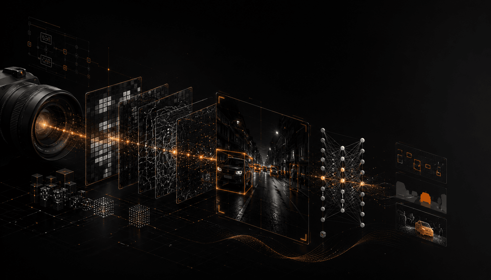
"Computer vision" gets discussed as though it were a single capability, but in practice it is a ladder of tasks, each answering a sharper question than the last. Show the same street photo to three systems and you can get three different kinds of answer: a car is in this image, or there is a car here and a cyclist there, or these exact pixels are car and those are road. Those are three distinct problems — classification, detection, and segmentation — and knowing which one you actually need is one of the most consequential early decisions in a vision project. This piece is the deeper dive that follows on from the mental model of computer vision: same foundation of pixels and learned features, now aimed at the three questions a vision system can answer.
Classification: what is in this image?
Classification is the entry rung. The model consumes the whole image and emits a single answer: one label, usually with a confidence score. "Cat." "Pneumonia." "Defective." Under the hood, a backbone network — a stack of convolutional layers — turns the pixel grid into a compact feature vector, and a small classifier head maps that vector to a probability across the possible classes.
The backbone is where most of the progress of the last decade lives. A recurring problem with early deep networks was that stacking more layers eventually made them harder to train, not better — the gradient signal degraded as it propagated back through many layers. Residual networks addressed this with skip connections: a layer learns a small adjustment to its input rather than a whole new transformation, and the input is added back on. That single idea let networks go much deeper without the training signal collapsing, and residual backbones became the default feature extractor that detection and segmentation models are built on top of.
Backbone
The feature-extraction portion of a vision model — typically a deep convolutional network — shared across tasks. Classification uses it directly; detection and segmentation bolt task-specific heads onto the same kind of backbone.
Classification is cheap because its labels are cheap: a human glances at an image and types one word. That economy is why it is the right tool whenever a single global answer is enough — is this X-ray normal, is this product photo the right category, is this frame safe to show.
Detection: what, and where?
The moment you need to know where something is, or to count multiple objects, you have moved to detection. The output is no longer one label but a set of bounding boxes, each with a class and a confidence. A single street scene might return a dozen boxes: several cars, two pedestrians, a traffic light.
Detectors come in two families, and the split is worth understanding because it maps directly onto a speed-versus-accuracy choice.
| Two-stage detectors | One-stage detectors | |
|---|---|---|
| How it works | First propose candidate regions, then classify and refine each | Predict boxes and classes across the image in a single pass |
| Representative line | R-CNN to Faster R-CNN (learned Region Proposal Network) | YOLO, SSD |
| Tends to be | More accurate, especially on small or crowded objects | Faster, often fast enough for real time |
| Good when | Accuracy matters more than latency | You need live throughput on video |
The two-stage lineage matured with Faster R-CNN, which replaced a slow, hand-designed region-proposal step with a small neural network — the Region Proposal Network — that learns where to look, sharing features with the classifier so the whole thing trains end to end. The one-stage lineage, exemplified by YOLO, reframed detection as a single regression over a grid: look once, predict every box in one forward pass. Historically that traded some accuracy for a large speed gain, which is exactly the right bargain for video and robotics.
# The shape of each task's output — what your downstream code consumes.

classification = {"label": "car", "confidence": 0.94}

detection = [
    {"label": "car",        "box": (x, y, w, h), "confidence": 0.94},
    {"label": "pedestrian", "box": (x, y, w, h), "confidence": 0.88},
]

# Segmentation returns a per-pixel label map the size of the image:
# segmentation[row][col] holds the class id for that pixel.
Segmentation: which pixels?
Segmentation is the most precise question: assign a label to every pixel. It comes in two flavours that are easy to conflate:
- Semantic segmentation labels each pixel by class but does not separate individual objects — all "car" pixels are simply "car", even if three cars overlap.
- Instance segmentation goes further, separating each object into its own mask, so you can count three distinct cars and outline each one.
The architectural workhorse for dense, pixel-level prediction is the encoder–decoder with skip connections. An encoder compresses the image down to deep features (losing spatial detail), then a decoder upsamples back to full resolution — and skip connections carry fine spatial information from the encoder across to the decoder so edges stay crisp. U-Net popularised this shape and remains widely used in biomedical imaging, where every pixel of a scan can matter. For instance segmentation, Mask R-CNN takes the detection machinery and adds a branch that predicts a mask inside each detected box — detection and segmentation fused into one model.
That progression is also a progression in labelling cost. A classification label is a word. A detection label is a box drawn by hand around every object. A segmentation label is a human tracing the outline of every object, pixel by pixel — slow, expensive, and the main reason segmentation datasets are smaller and pricier than classification ones.
Choosing the right task
The common early mistake is reaching for more precision than the problem needs, and paying for it in labels and latency forever after.
Pros
- Classification: cheapest labels, smallest models, fastest to ship when one global answer suffices.
- Detection: locates and counts objects; mature tooling; a clear speed/accuracy dial between one- and two-stage families.
- Segmentation: pixel-exact boundaries, essential for medical imaging, editing, and measurement.
Cons
- Classification: tells you nothing about where or how many.
- Detection: boxes are coarse — they include background around odd shapes, and crowded scenes are hard.
- Segmentation: labels are the most expensive to produce and the models the most demanding to train and run.
Ask what the downstream system actually consumes
If the next step in your pipeline only needs to know a photo's category, do not label ten thousand bounding boxes. If it needs to measure the area of a tumour, a box will not do — you need a mask. Let the real consumer of the output pick the task, not the other way round.
Practical takeaway
Classification, detection, and segmentation form a ladder of rising specificity — a single label, then labelled boxes, then a per-pixel map — and each rung costs more to label and more to run than the one below it. The model families are largely settled and downloadable: residual backbones for classification, the two-stage and one-stage detector lineages for boxes, encoder–decoder and mask-branch architectures for pixels. The engineering judgement that still matters is choosing the lowest rung that answers your question, and then investing your effort in labels that resemble the messy reality your system will actually see.
Sources & Further Reading
- 01Deep Residual Learning for Image Recognition (ResNet) — He, Zhang, Ren & Sun, 2015Skip connections that made very deep classification backbones trainable.
- 02Faster R-CNN: Towards Real-Time Object Detection with Region Proposal Networks — Ren, He, Girshick & Sun, 2015The learned region-proposal step behind two-stage detectors.
- 03You Only Look Once: Unified, Real-Time Object Detection (YOLO) — Redmon, Divvala, Girshick & Farhadi, 2015Detection as a single-pass regression — the one-stage family.
- 04Mask R-CNN — He, Gkioxari, Dollár & Girshick, 2017Adds a per-object mask branch for instance segmentation.
- 05U-Net: Convolutional Networks for Biomedical Image Segmentation — Ronneberger, Fischer & Brox, 2015The encoder–decoder with skip connections for dense prediction.
- 06CS231n: Convolutional Neural Networks for Visual Recognition — Stanford UniversityCourse notes covering all three task families.
Editorial note — A conceptual explainer on established computer-vision task types and the model families behind them. Architectures are described qualitatively; no benchmark scores, speeds, or accuracy figures are quoted.