If you feed an image to an ordinary fully-connected neural network, you immediately hit two problems: the number of weights explodes, and the network has no built-in notion that a cat in the top-left corner is the same cat when it moves to the bottom-right. Convolutional neural networks solve both by building assumptions about images directly into their structure. That architectural head start is why, for more than a decade, they have been the default tool for vision. This is a look under the hood at what a convolutional network actually is, and why its design fits images so well.
Why not just use a normal network?
Picture connecting every pixel of a modest image to every neuron in a first hidden layer. A million-pixel image and a thousand neurons is already a billion weights in one layer — unlearnable, and hopelessly prone to overfitting. Worse, a fully-connected layer treats each pixel position as unrelated to its neighbours, so it has to learn the concept of "edge" separately for every location it might appear in.
Both problems come from ignoring what we know about images. Two facts stand out. First, visual structure is local: whether a small patch is an edge depends only on the pixels in that patch, not on a pixel across the image. Second, a good feature detector is position-independent: an edge detector that works in one corner works everywhere. A convolutional network encodes both facts into its wiring.
The convolution layer
The core building block slides a small grid of weights — a filter or kernel, perhaps 3-by-3 — across the image, computing a weighted sum at each position to produce an output grid called a feature map. Because the same filter is used at every position, the network learns one set of weights and reuses it everywhere. This is weight sharing, and it is the source of the CNN's efficiency: a 3-by-3 filter is nine weights regardless of image size, and it automatically detects its pattern wherever that pattern occurs.
Three knobs shape the output:
- 1
Filters (depth)
Each layer learns many filters, each producing its own feature map — one might fire on vertical edges, another on a particular colour or texture. The stack of feature maps is the layer's output.
- 2
Stride
How far the filter jumps between positions. A stride of one looks everywhere; a larger stride skips positions and shrinks the output, downsampling as it goes.
- 3
Padding
Whether to pad the border with zeros so the output keeps the input's size. Without padding, each convolution nibbles pixels off the edges.
There is a simple formula for how a layer changes spatial size. For an input of size N, a filter of size F, padding P, and stride S, the output side length is (N - F + 2P) / S + 1. It is worth internalising, because it is how you reason about what a network does to an image's dimensions as it flows through.
Input 32x32, filter 3x3, padding 1, stride 1:
  (32 - 3 + 2*1) / 1 + 1 = 32   -> size preserved (padding keeps the border)

Input 32x32, filter 3x3, padding 0, stride 2:
  (32 - 3 + 0) / 2 + 1 = 15     -> downsampled by the stride
Pooling and the feature hierarchy
Interleaved with convolutions is pooling, which downsamples a feature map by summarising small regions — max pooling keeps the strongest response in each little window. Pooling shrinks the spatial dimensions (cutting computation and adding a bit of tolerance to small shifts) while the number of feature maps typically grows. The image gets smaller and deeper as it advances.
That progression builds a hierarchy of features, and it is the most important idea to hold onto. Early layers, seeing only small patches, learn simple things: edges, colours, gradients. Middle layers combine those into textures and motifs. Late layers, whose neurons indirectly see a large portion of the original image, respond to whole object parts and objects. This growing window is the receptive field: the region of the input that influences a given neuron, which expands layer by layer until deep neurons effectively see the whole scene.
Depth, and the problem it created
If depth builds richer features, why not stack layers without limit? Because for a long time, deeper networks became harder to train — beyond a point, adding layers made accuracy worse, as the gradient signal used to train early layers degraded on its way back through many layers. This was a genuine obstacle, not merely a matter of compute.
The lineage of architectures is largely a story of pushing depth. Early convolutional networks were shallow. The 2012 ImageNet result brought a notably deeper network and, with it, the shift to learned features across the whole field. Subsequent designs went deeper still with small, uniform filters. The decisive fix for the training problem was the residual connection: instead of asking a block of layers to produce a whole new representation, you ask it to learn a small adjustment and add that to its input. The unmodified input takes a shortcut around the block, so the training signal has a clean path backwards no matter how deep the network is. Residual networks made very deep models routine, and their design still underpins a large share of vision backbones today.
Depth builds abstraction — but only if it trains
The value of a deep network is the hierarchy it can represent: simple features composing into complex ones. That value is only realisable if the gradient can reach the early layers. Skip connections were the architectural trick that reconciled 'go deeper' with 'stay trainable'.
Transfer learning: the practical payoff
Here is the fact that changes day-to-day practice: the early and middle layers of a network trained on a large, diverse image set learn general-purpose features — edges, textures, shapes — that transfer to almost any vision task. So you rarely train from scratch. You take a pretrained backbone, keep its learned features, and fine-tune a small head on your own (often much smaller) dataset. This is transfer learning, and it is why a team with a few thousand labelled images can still build a strong classifier: they are standing on features learned from millions.
Practical takeaway
A convolutional network is not a mysterious black box so much as a set of well-chosen assumptions made concrete: features are local, so look at small patches; a good feature is useful anywhere, so share weights across positions; complex structure is built from simple structure, so stack layers into a hierarchy. Pooling manages size, the receptive field grows until deep neurons see the whole image, and residual connections keep the whole thing trainable at depth. In practice you will rarely build one from nothing — you will fine-tune a pretrained backbone — but knowing what each part is doing is what lets you diagnose a model that is not learning what you hoped.
Sources & Further Reading
- 01Deep Residual Learning for Image Recognition (ResNet) — He, Zhang, Ren & Sun, 2015Skip connections that made very deep CNNs trainable.
- 02Deep Learning, Ch. 9: Convolutional Networks — Goodfellow, Bengio & Courville, 2016The theory of convolution, pooling, and parameter sharing.
- 03CS231n: Convolutional Neural Networks for Visual Recognition — Stanford UniversityThe standard course notes on CNN architecture and training.
- 04ImageNet Large Scale Visual Recognition Challenge — Russakovsky et al., 2015The benchmark whose 2012 results triggered the deep-learning shift in vision.
Editorial note — A conceptual explainer on established convolutional-network architecture. The 2012 ImageNet milestone is described qualitatively; no accuracy figures, parameter counts, or benchmark numbers are quoted.