Long before deep learning, engineers were already doing remarkable things with images using nothing but arithmetic on a grid of numbers. That body of work — classical image processing — has not gone away. It is what runs when your phone sharpens a photo, what cleans up a scanned document before text recognition, and what a vision pipeline often uses to prepare an image before any model touches it. It is fast, deterministic, and completely explainable, which is exactly why it remains the right tool for a large class of problems. This is a tour of the core operations, built up from the pixel.
The substrate: pixels, channels, histograms
Start where every image starts: a two-dimensional array of intensity values, one per pixel, from 0 (black) to 255 (white) for an 8-bit grayscale image. A colour image is three such arrays — red, green, blue — stacked. Everything below is a function that takes this grid and returns another grid, or a summary of it.
A useful summary is the histogram: a count of how many pixels fall at each intensity level. It says nothing about where things are, only how bright the image is overall — but that is enough to reason about exposure. A photo bunched up at the dark end is underexposed; spreading that distribution out across the full range (contrast stretching, or histogram equalisation) is one of the oldest and most effective enhancements there is.
Point operations: one pixel at a time
The simplest transforms treat each pixel independently — the output at a location depends only on the input at that same location. These are point operations, and they cover a surprising amount of ground:
- Brightness — add a constant to every pixel.
- Contrast — scale every pixel around a midpoint, pushing lights lighter and darks darker.
- Gamma correction — apply a non-linear curve, because both displays and human perception of brightness are non-linear.
- Thresholding — map everything above a cutoff to white and everything below to black, turning a grayscale image into a binary one. This is the classic first step in isolating an object from its background.
import numpy as np

def adjust(img, brightness=0, contrast=1.0):
    # img: a 2D array of pixel values in [0, 255].
    out = img.astype(float) * contrast + brightness
    return np.clip(out, 0, 255).astype(np.uint8)   # keep values in range

def threshold(img, cutoff=128):
    # Everything at or above the cutoff becomes white; the rest black.
    return np.where(img >= cutoff, 255, 0).astype(np.uint8)
Because point operations ignore a pixel's neighbours, they cannot blur, sharpen, or find edges. For that you need to look around.
Neighbourhood operations: convolution
The workhorse of spatial processing is convolution: slide a small grid of weights — a kernel — over the image, and at each position multiply the kernel against the pixels beneath it and sum the result to produce one output pixel. Change the kernel and you change the operation entirely.
| Kernel intent | What it does | Effect |
|---|---|---|
| Averaging / Gaussian | Blends each pixel with its neighbours | Blur, noise reduction |
| Difference (e.g. Sobel) | Responds to rapid intensity change | Edge detection |
| Sharpening | Amplifies the difference from the local average | Crisper detail |
A blur kernel is just a small patch of positive weights that averages a neighbourhood — smoothing out noise at the cost of fine detail. An edge kernel does the opposite: it responds where brightness changes fast, because an edge is a rapid change in intensity. This is precisely the operation covered in more depth in the computer-vision explainer — and it is the same operation a convolutional network later learns to perform with kernels discovered from data rather than designed by hand.
The through-line to deep learning
Classical vision hand-designs kernels: Sobel for edges, Gaussian for blur. A convolutional neural network keeps the convolution but learns the kernel weights from labelled examples. The mechanism is identical; only the source of the numbers changed.
Binary images and morphology
Once you have thresholded an image down to black and white, a family of shape-based operations called morphology cleans it up. The two primitives are erosion (shrink the white regions, which removes small specks of noise) and dilation (grow them, which fills small holes). Compose them and you get opening (erode then dilate, to remove noise while keeping overall size) and closing (dilate then erode, to seal gaps). These are the humble, reliable operations behind tidying up a scanned form or a segmentation mask before anything downstream consumes it.
Colour spaces
RGB is how images are usually stored, but it is often the wrong space to work in, because brightness and colour are tangled across all three channels. Converting to a space that separates them — such as HSV (hue, saturation, value) or a luma/chroma space — makes many tasks far easier. Want to select "all the reddish pixels regardless of lighting"? That is awkward in RGB and natural in a space where hue is its own axis. Choosing the right colour space is often more than half the battle in a classical pipeline.
When classical beats learned
Pros
- No training data, no labels, no GPU — often just a few lines of array math.
- Deterministic and fully explainable: you can point at exactly why an output looks the way it does.
- Fast and cheap enough to run in real time on modest hardware, ideal for preprocessing.
Cons
- Struggles with high-level semantics — 'is this a cat?' is not a filter.
- Sensitive to tuning: thresholds and kernel sizes often need hand-adjustment per dataset.
- Hits a ceiling on messy, variable real-world scenes where learned features shine.
The honest framing is that classical and learned methods are partners, not rivals. Deterministic processing dominates the low-level, well-defined jobs — denoise, deblur, normalise, threshold, clean up — and it frequently runs as the preprocessing step that feeds a learned model. Reach for a network when the task is semantic and variable; reach for a kernel when it is geometric and well-specified.
Practical takeaway
Classical image processing is worth learning even in a deep-learning era, because it is the layer that turns raw, noisy pixels into something a model — or a human — can use, and it does so transparently. Build the mental library: histograms for exposure, point operations for per-pixel adjustments, convolution for anything spatial, morphology for cleaning up binary masks, and the right colour space to make a hard task easy. Most of the time, when an image looks wrong going into a system, one of these deterministic tools is the fastest, most debuggable way to fix it.
Sources & Further Reading
- 01Computer Vision: Algorithms and Applications (2nd ed.) — Richard Szeliski, 2022Free reference covering classical processing alongside modern methods.
- 02OpenCV Documentation — Image Processing modules — OpenCVReference and tutorials for filtering, morphology, thresholding, and colour spaces.
- 03Canvas API — pixel manipulation — MDN Web DocsHow to read and transform pixel data directly in the browser.
Editorial note — A conceptual explainer of established, deterministic image-processing techniques. Code is illustrative; no benchmark figures or dataset-specific results are quoted.